The Jeffreys Prior
Suppose you know that some repeatable binary event (like a coin flip coming up heads) has a probability $p\in[0,1]$ of occurring. You have no idea what $p$ is, and you’d like to make an estimate. Using a bunch of experiments to get data ${data}$, and following Bayes theorem, we obtain a distribution over $p$ values of:
\[P(p|\{data\}) = \frac{P(\{data\}|p)Prior(p)}{P(\{data\})}\]This all sounds good, but hold on… how do we know what this thing “$Prior(p)$” should be? I already said I have no idea what $p$ is, but by specifying $Prior(p)$, I’m saying “psych, I actually do have some beliefs about it”.
Where does this prior, $Prior(p)$ come from? What is $Prior(p)$?
Basically, the question is, how do you form a prior for some parameter $p$, when you have absolutely no idea what $p$ should be. How do you mathematically state your beliefs when you have none; when you are in a state of “maximal ignorance”.
Jeffreys’s Argument The Argument of Jeffreys
There’s a natural assumption at this point that you should simply treat every probability as equally possible:
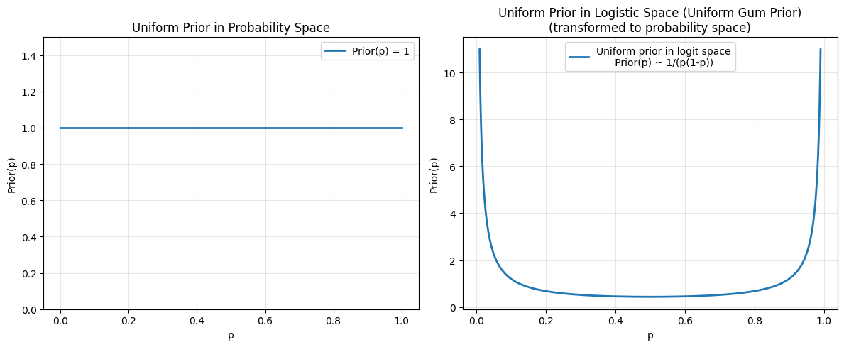
\[Prior(p) = 1\]If this feels right to you, you’re in good company. Apparently even Laplace (of transform fame) thought this was correct: If you have no preference for one probability over another ($p=.3$ vs $p=.5$ for instance), then surely you should give them the same prior value ($Prior(.3)=Prior(.5)=Prior(p)=1$ after normalizing for $p \in [0,1]$). The prior about your coin’s probability of heads should just be a constant.
But then Jeffreys (yes, his name is a plural) came along and asked, “hey, what if somebody’s been adding chewing gum to the tails or heads side of a fair coin? And what if an amount of chewing gum, $g$, stuck to the tails side ($g>0$) or heads side ($g<0$) causes the probability of heads ($p_h$) to become
\[p_h(g) = \frac{1}{e^{-g} +1}\]We know nothing about how much gum was stuck to this thing. What should my maximal ignorance prior over $g$ be?”
I mean obviously he didn’t say this, but the idea is that you don’t have to use a number between 0 and 1 to parametrize a probability. You could use $g$ (called logits, and never “gum weight”), you could even use $1/p$. Gum weight parametrization $g$ is just as effective as $p$, So why would the flat prior in $p$ be the right one? What about the flat prior over gum – saying that every logit, $g$, is equally likely?
The answer is that your maximal ignorance prior shouldn’t depend on your parametrization. In fact, if you said one parametrization was “better” than another (choosing $p$ vs $g$), then you’d be bringing some beliefs to this problem (beliefs like “that whole ‘gum weight’ analogy you wasted my time with was dumb”), and so you would immediately be failing in your goal of maximal ignorance.
A Non-Explanation
Jeffreys said that the solution is to use a quantity which is invariant under reparametrization, namely the square root of the Fisher information: $\sqrt{\mathcal{I}(\theta)}$ (where $\theta$ is whatever parametrization you’re currently using), because
\[\sqrt{\mathcal{I}(\theta)} d\theta = \sqrt{\mathcal{I}(\phi)} \left|\frac{d\theta}{d\phi}\right| d\phi\]Therefore the Jeffreys prior is
\[Prior(p) \propto \sqrt{\mathcal{I}(p)}\]And done, you now know the Jeffreys prior goodbye, have a nice evening.
This is basically where every tutorial I’ve seen about the Jeffreys prior ends. They just kind of tell you that the square root of the Fisher information is invariant under reparameterization, maybe they give a uniqueness theorem, and then they pat you on the back and send you to bed because you have now learned that Jeffrey’s prior is the square root of the Fisher information and all questions are thus answered.
This always pisses me off because we’re left with a proof that it’s right, but utterly no understanding.
Now if you already know what the square root of the Fisher information represents, then sure, this explanation is fine. But if you don’t, then this explanation is useless to you. This is how a lot of math textbooks are: obviously written by people who have already gotten to the point of understanding everything, but have seemingly forgotten exactly how they got there.
An Explanation
I prefer a different explanation of the Jeffreys prior. I came up with this while explaining it a few years back. I’m sure that it’s somewhere online but I haven’t seen it exactly like this, and having done no research at all, I think with maximum ignorance I can assert that this explanation is mine.
Let’s go back to the problem of choosing a prior for the probability of a coin coming up heads. I’m going to call each probability of heads, $p$, a “theory”. We’re still totally on board with the idea that each distinct theory is equally probable, since we still have no reason to choose one theory over a different one.
Listing Out the “Different” p’s
First though, we have to define what we mean by “different”. Let’s get concrete: let’s say that a theory $p+\epsilon$ is “different” from $p$, if by looking at $N$ coin flips from $p$, I can with some fixed degree of confidence say that this data does NOT come from $p+\epsilon$.
It turns out this is related to a quantity called the KL divergence by \(N \sim 1/KL(p\|q)\) where \(KL(p\|q) = \sum_x p(x) \log(p(x)/q(x))\) and $x$ is every ‘event’ which can occur (here, a head or a tail). (For continuous events, we integrate)
If you know what KL divergence is, then this is still neat, but almost a tautology. In a very rigorous way, the KL divergence tells you how much extra “surprise” you should get from your data if you think it comes from $q$, but it actually comes from $p$. Here, “surprise” is measured in nats (bits in base $e$). 1
Intuitively (and actually), on average each experiment will give you the same amount of nats of information \(KL(p\|q)\). So If you specify a fixed surprise threshold, $S$, then the number of experiments you require ($N$) should obey
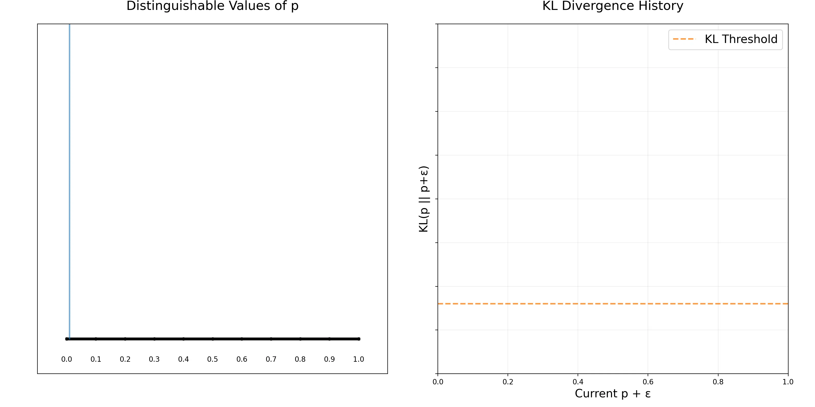
\[S \sim N \cdot KL(p\|q) \text{ and so } N \sim 1/KL(p\|q)\]Great! Now we can do a little math and get a big bucket of distinguishable theories by finding the smallest epsilon so that \(KL(p\|p+\epsilon) = threshold\).
Choosing From the p’s
Now that I’ve really listed out all the possible distinguishable theories, I can actually go about choosing one with maximum ignorance - that is, I can take one $p$ from this bucket of different theories totally at random. This is the correct way to form your maximum ignorance prior over $p$.
The Resulting Prior(p)
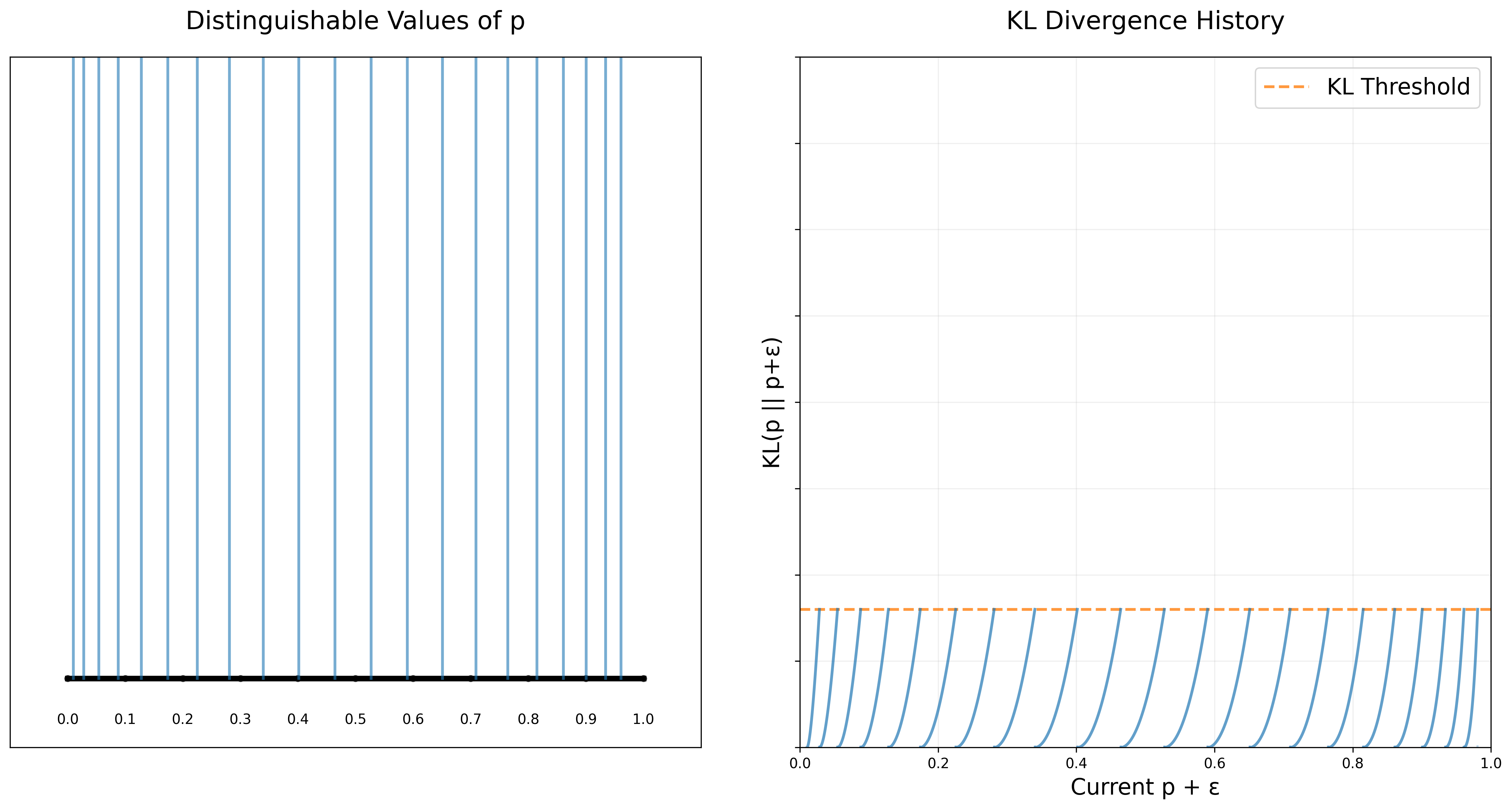
If we look at this plot of different theories, we can see that they aren’t uniformly spaced. It looks like there are more theories near 0 and 1. Something interesting is going on.
I want a concrete formula for $Prior(p)$, so Let’s get more precise, and take $N$ (the number of times we can flip the coin) to infinity. Our theories $p$ and $p+\epsilon$ are going to be pretty close together, so we do a little math (Taylor expanding) and find that for small $\epsilon$,
\[KL(p\|p+\epsilon) = \frac{\epsilon^2}{2p(1-p)}\]And so, setting $KL(p|p+\epsilon)$ equal to a constant small surprise threshold, $S$, gives us:
\[S = \frac{\epsilon^2}{2p(1-p)}\]The density of distinguishable theories is then going to be $\sim 1/$(distance between theories) $\sim 1/\epsilon$. A little rearranging shows that \(Prior(p) \sim 1/\epsilon \sim \frac{1}{\sqrt{p(1-p)}}\)
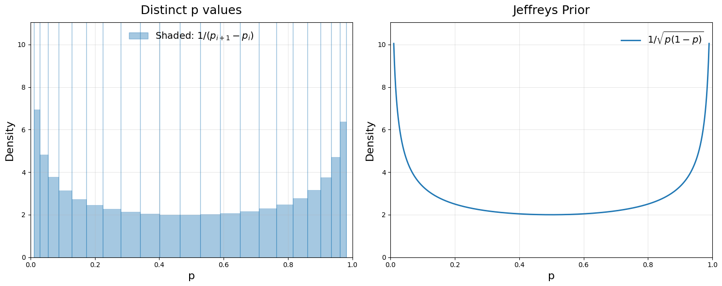
There we have it – the density of distinguishable theories. A sample from this distribution gives us the Jeffreys prior.
Full Circle
If we think a little harder about this plot, we can finally go full circle.
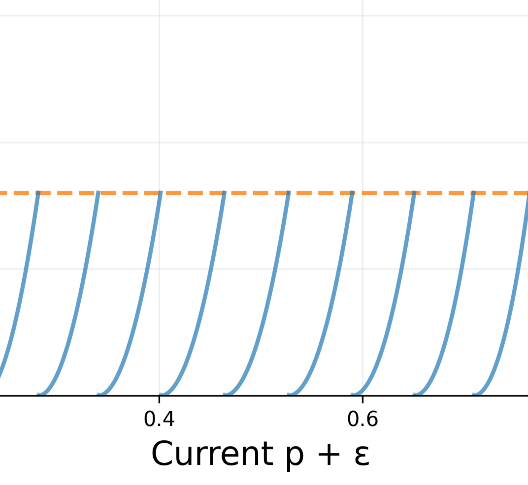
we can see that each one of these curves is kind of like a parabola. I say “kind of like”, but we can make this rigorous. If we evaluate the taylor series here, we get
\[KL(p, p+\epsilon) \approx KL(p\| p) + \epsilon \left(\frac{dKL(p\| q)}{dq}\right)\bigg|_{q=p} + \frac{\epsilon^2}{2} \left(\frac{d^2KL(p\| q)}{dq^2}\right)\bigg|_{q=p}\]now we can simplify. Here I’m going to overload $p$ as denoting both the parameter of the probability, and the probability distribution function itself $p(x)$:
\[KL(p\| p) = 0\] \[\left(\frac{dKL(p\| q)}{dq}\right)\bigg|_{q=p} = \frac{d}{dq} \left(\sum_x p(x) \log(p(x) / q(x))\right)\bigg|_{q=p} = - \left(\sum_x p'(x)\right) = -\frac{d}{dp} \left(\sum_x p(x)\right) = -\frac{d}{dp} 1 = 0\]Now we have the second order parabolic term. We need to massage this one a tiny bit, but without too much trouble we get that
\[\left(\frac{d^2KL(p\| q)}{dq^2}\right)\bigg|_{q=p} = \sum_x p(x) \left(\frac{p'(x)}{p(x)}\right)^2 = \sum_x p(x) \left(\frac{d}{dp} \log(p(x))\right)^2\]This last term has another name, the Fisher Information:
\[\mathcal{I}(\theta) = \sum_x p(x) \left(\frac{d}{d\theta} \log(p_{\theta}(x))\right)^2\]So the taylor expansion to second order reduces to
\[KL(p\|p+\epsilon) \approx \frac{1}{2} \mathcal{I}(p) \epsilon^2\]Because the previous terms are zero, the Fisher information $\mathcal{I}(p)$ totally defines $KL(p| p+ \epsilon)$ for small $\epsilon$.
And so in general, fixing a KL divergence threshold gives us a density of prior probabilities of
\[Prior(p) \sim 1/\epsilon \sim \sqrt{\mathcal{I}(p)}\]Which brings us back to the claim of that proofy, non-explanation we initially saw, but now we know why. Specifically, $\sqrt{\mathcal{I}(p)}$ tells us how ‘quickly’ the theories change at a point $p$. It’s like the natural volume element in theory-space – a sort of minimal pixel size of a theory as a function of its parameters – which tells us how much a theory changes as you vary them.
Our initial flaw (and Laplace’s) in assuming that every probability was equally likely ($Prior(p)=1$), was in using the wrong metric. In reality, theories can ‘bunch up’ in certain areas of parameter space. It’s as if we tried to do an opinion poll of the US by sampling one person per 500 square miles. We’d only get one person from NYC, even though it makes up $\sim 3\%$ of the US.
Extra Nats of Information
Like a lot of great fields in math and physics, information theory has the tendency to feel obvious once you understand it. Even famous results with famous names can seem so inevitable that it seems almost silly to write them down.
For example, the Cramer-Rao bound. This is an immensely important result. Suppose you have some model of an event, $p_{\theta}(x)$. You’re running experiments to try to find out what the current $\theta$ is (sound familiar?). It tells us that given $N$ experiments, the variance in your estimate, $\hat{\theta}$, of the model parameter has a familiar lower bound:
\(\text{Var}(\hat{\theta}) \geq \frac{1}{N \mathcal{I}(\theta)}\)2
But knowing what we know, wouldn’t we almost guess this? After $N$ experiments, you have
\[KL(p\|p+\epsilon) \approx \frac{1}{2} N \mathcal{I}(\theta) \epsilon^2\]Therefore the ‘resolution’ of theory space with $N$ experiments is $\propto 1/\sqrt{N \mathcal{I}(\theta)}$. A rough estimate of the uncertainty given that $p$ and $p+\epsilon$ are just as good tells you
\[\text{Min}(\text{Var}(\hat{\theta})) \propto (\epsilon/2)^2 \propto \frac{1}{N \mathcal{I}(\theta)}\]The ‘result’ part of the Cramer-Rao bound just seems to be the constant (1) that they place on this relationship.
The more you learn about information theory, the more inevitable and interrelated it feels, which is a lot of fun.
A note about the banner to this article
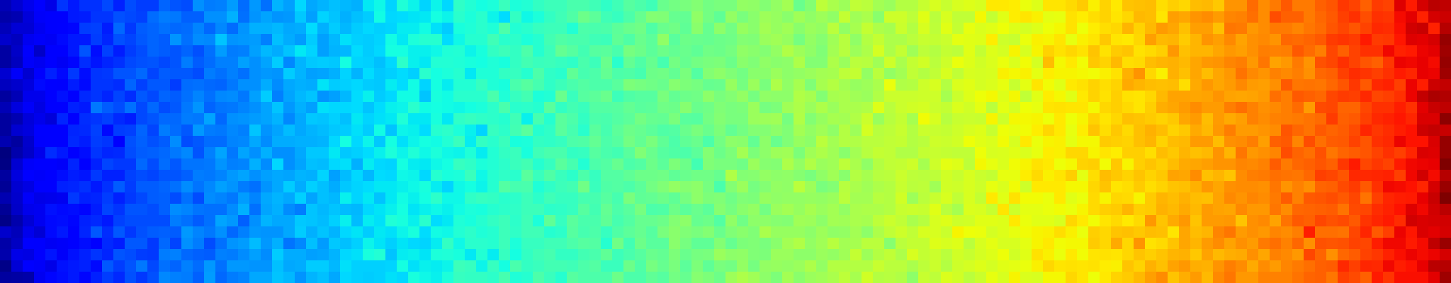
It turns out that there is one parametrization $\phi$ of the coin flip probabilities, in which changing the parameters by a constant amount $\Delta \phi$ changes the resulting theory by a constant amount:
\(\phi = \arcsin(\sqrt{p})\) which satisfies \(\frac{d \phi}{d p} \propto \sqrt{I(p)}\)
Here, the pixels are colored using the jet colormap, but chosen as a function of $\phi(p)$, where $p$ is the fraction of the way through the banner. Scaling $\phi_{\min}$ and $\phi_{\max}$ to the colormap’s start and stop, and adding in a tiny bit of noise (for fun), we can see how changing $p$ by a constant amount actually modifies the resulting theory (the colors). We sweep through the colors quickly near the edges (the dark blue on the left and dark red on the right are barely there), but near $p=1/2$ (the middle) the colors are stretched out, and the theories are less dense.
Footnotes
1: One of the first mind-blowing information theory facts I learned in undergrad was that surprise is in fact a rigorous concept (see information content).
2: We’re saying a single experiment has fisher information $\mathcal{I}(\theta)$, then $N$ repetitions contributes $N \mathcal{I}(\theta)$.