
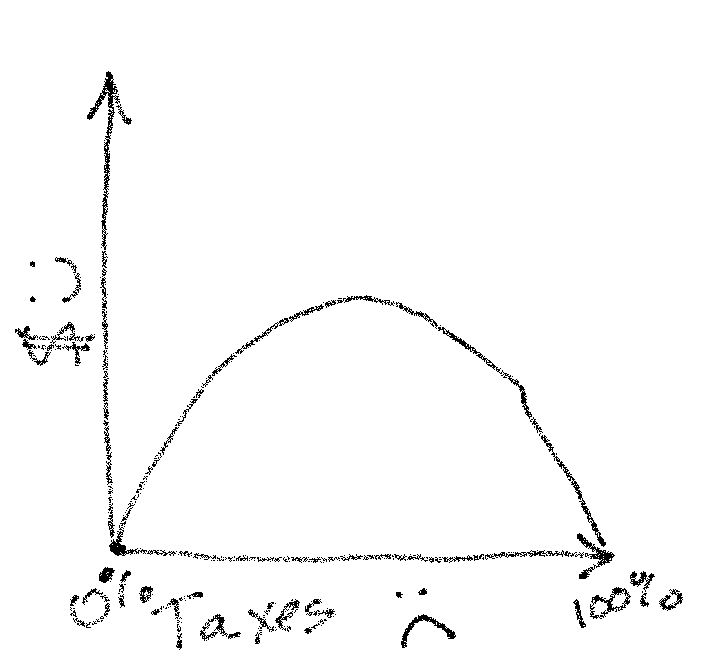
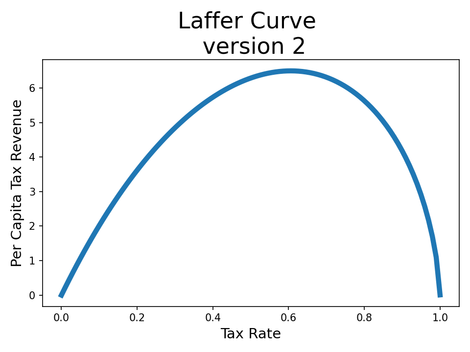
I started this project because I wanted to reproduce the Laffer curve – this is a very famous plot showing tax revenue vs tax rate. Here’s the summary:
1) $t\rightarrow 0$: When the tax rate is zero, the government gets no revenue, because it collects nothing.
2) $t\rightarrow 1$: Now as the tax rate reaches 1, nobody works (because they get to keep nothing they earn) and so again the government gets no revenue.
3) $0<t<1$: Here, people keep some of what they earn, and so they are incentivized to work. Meanwhile, the government gets a cut as well.
Whenever I hear about the Laffer curve, it’s usually described at this level - usually there’s a story involving Laffer drawing something like a graph on a napkin for Reagan or somebody.
I have no idea why it got named after Laffer, because there’s no way he was the first person to realize something so obvious. A quick glance at wikipedia indicates that he was the first person to claim that we were on the descending side of the peak – which would just be so unbelievably convenient to believe if you were a rich guy in the 70s who already wanted taxes to be lower.
Anyway, I want to see if I could observe the Laffer curve from some kind of first-principles argument, rather than just an intuitive napkin-sketch.
Basically, I want to look at some of the effects of simulated taxes applied to a simulated population.
We’ll begin with a super simple toy model for an economy and add complexity from there.
Personal Utility Function: $U(x)$
Our first step is to have some way of determining how much each person works. To figure this out, we need to put together a utility function for each person, which takes as an input how much that person works.
Let’s define the building blocks:
-
$B(z)$: The utility gained from getting income $z$ \(B(z) = \beta \log(z)\) ($\beta$ is like greed). I’m making this Logarithmic because that’s roughly how people’s happiness seems to respond to incomes. Initially I was thinking of making this function $\propto \log(z+1)$ – meaning that when you have no income, you get zero happiness. But I think a more accurate function would reflect that zero income doesn’t just contribute 0 utility, it means you’re destitute and living on the sidewalk (which I would guess is not too far from $-\infty$)
-
$m(x)$: the amount of money earned by an individual exerting themself a degree $x$ We’ll say that \(m(x) = s x\) Here, $s$ is like skill, and $x$ is basically how much they’re working.
-
$C(x)$: The personal cost of working an amount $x$ \(C(x) = \gamma x\) ($\gamma$ is like laziness, or how much you hate doing your job)
-
$t$: A flat tax rate (flat for simplicity), which tells us what fraction of a person’s salary the government takes.
Computing Production
Now let’s figure out how much each person will work: $x^*$
We expect people will maximize their utility - exerting themselves until they feel it is no longer worth it. Of course, everyone has the choice to not work at all, and nobody works a negative amount. Therefore we can write:
\[x^* = \max(0, \text{argmax}_{x} U(x))\]Since $U$ is concave, we can solve this by setting the derivative to zero.
\[x^* = \max(0, x^* \ s.t. \ \frac{dU}{dx}|_{x^*} = 0)\]Utility Version 0
As our simplest possible model, let’s use the following (bleak) assumptions:
- flat tax rate: everyone has a fraction $t$ of their earnings taken
- taxes = pure theft: the revenue the government collects from you through taxes contributes nothing to your life. This also means that there’s no social safety net. The only way anyone gets income is by working
- everybody is a clone: All parameters are the same for each person in the society
This gives us \(U(x) = \beta \log((1-t)sx) - \gamma x\)
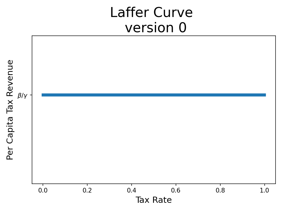
Interestingly, here it doesn’t matter what the tax rate is. Whatever the government taxes us, we will be working an amount \(x^* = \beta / \gamma\) The only effect that taxes have here is to make everyone sadder :(.
\[U(x) = \beta \log((1-t)sx) - \gamma x = \beta \log(sx) - \gamma x + \beta \log(1-t) = U_{t=0}(x) - |\beta \log(1-t)|\] \[U(x) = U_{t=0}(x) - |\beta \log(1-t)|\]Let’s introduce a little complexity to see how we can make this more interesting
Utility Version 1
As our next simplest possible model, let’s make a change. As before
- flat tax rate: everyone has a fraction $t$ of their earnings taken from you
- everybody is a clone: All parameters are the same for each person in society
But now
- tax and dividend: to model services that the government provides all the citizens, we’ll say that whatever the government collects in taxes is returned in equal parts to each person. For short, I’ll refer to this as a UBI (universal basic income), although maybe this takes the form of welfare + roads/bridges + public school etc.
This gives us \(U(x) = \beta \log(t\langle s x \rangle + (1-t)sx) - \gamma x\) Where the UBI, $t \langle s x \rangle$, is the tax rate $t$ multiplied by each person’s income, divided by the population. In other words, it is $t$ times the average production per person.
But notice that because everybody is identical, $\langle s x \rangle = s x$, and so taxes do nothing. \(U(x) = \beta \log(sx) - \gamma x\)
Obviously we need another ingredient
Utility Version 2
To make this interesting, we need to introduce some variance in the population. We’ll say that skill, $s$, is distributed log-normally within the population.
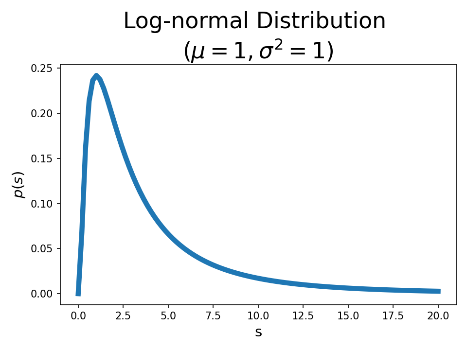
This probably isn’t too far from reality, where some people can earn many times more than the median person. Of course in the real world, greed ($\beta$) and laziness ($\gamma$) would vary as well, but I want to keep things as simple as possible.
Now each individual’s utility function isn’t so trivial: \(U(x) = \beta \log(t\langle s x \rangle + (1-t)sx) - \gamma x\)
Let’s solve for the amount each person will work, as a function of their skill \(x^*(s) = \max(0, x^* \ s.t. \ \frac{dU}{dx}|_{x^*} = 0) = max(0, \frac{\beta}{\gamma} - \frac{t\langle s x \rangle}{(1-t)s})\)
Self-consistency
The problem now is that how much each person works is a function of how much UBI income they get, but the UBI income they get is a function of how much each person works. So we need to find the self-consistent solution here. We’ll assume some log-normal parameters $\mu$ and $\sigma$ for the distribution of $s$ in the population, and try to find it.
For this to be self-consistent, we need the expectation to actually match the value it should have:
\[\langle s x^*(s) \rangle = \langle \max\big(0, \frac{s\beta}{\gamma} - \frac{t \langle s x \rangle}{1-t}\big)\rangle = \int_0^{\infty} ds \ \max\big(0, \frac{s\beta}{\gamma} - \frac{ t \langle s x \rangle}{1-t}\big) p_{\mu, \sigma}(s)\]Or
\[\langle s x^*(s) \rangle = \int_{s_{min}}^{\infty} ds \ \left(\frac{s\beta}{\gamma} - \frac{t \langle s x \rangle}{1-t}\right) p_{\mu, \sigma}(s), \quad s_{min} = \frac{t \langle s x \rangle}{1-t}\frac{\gamma}{\beta}\]Basically, we need for $\langle s x^*(s) \rangle$ to match $\langle s x \rangle$.
Practically, we can do this by plugging in some temporary value for the mean production, $\langle s x \rangle$, $\lambda$, and sweeping over $\lambda$ until it matches the self-consistent value of $\langle s x^*(s) \rangle$.
\[\langle s x^*(s) \rangle_{\lambda} = \langle \max\big(0, \frac{s\beta}{\gamma} - \frac{t \lambda}{1-t}\big)\rangle\]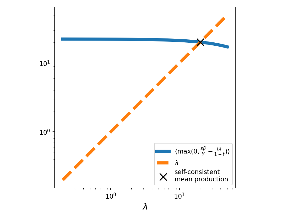
Laffer Curve
Now that we have a way to solve for this, we can compute whatever we want.
Let’s start with what we originally wanted to compute: the Laffer curve – the mean revenue collected by the government, as a function of tax rate.
Now let’s compute something else: instead of asking for the revenue as a function of tax rate, let’s compute the mean utility as a function of tax rate.
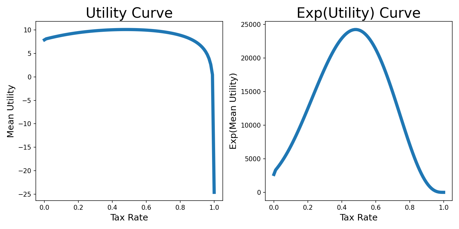
This is very log-y and so it’s pretty flat, so I’ve added the plot of the exp(mean utility) to the right to show the peak more.
Here, low tax rates mean the least well-off people get no government assistance, and so they’re forced to work more. This is a bit of a bummer. But what’s even more of a bummer is when the government takes all of everyone’s income. Here, nobody is rewarded much for working – why would you work when somebody’s taking basically all that you earn – and so tax revenue drops to zero, and so UBI drops to zero as well. The resulting situation is that everything sucks for everyone.
Another interesting result of flat tax+UBI here is that sometimes, you shouldn’t work at all. Working just isn’t worth your time when there’s the option of not working and receiving some government cheese. Note this only happens in this model because happiness due to income has diminishing returns ($\beta log(\text{income})$ is concave) while how much it sucks to work is linear ($-\gamma x$).
Let’s plot the lowest income rate (skill level, $s$) where working is just barely worthwhile vs the fraction of income kept (this is $1-t$).
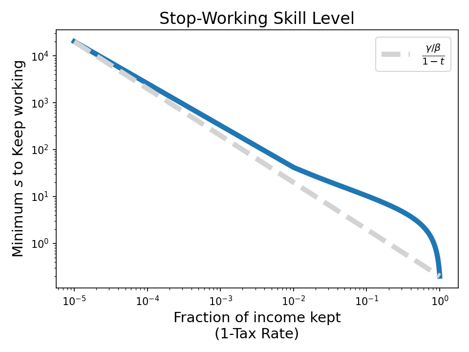
Note that as the tax rate drops to zero, everyone’s working, regardless of skill level
One final question
Suppose all we care about is minimizing the suffering of the poorest people – Under this model, this means we want to maximize per capita tax revenue, since this goes right back into everyone’s pockets – in particular, the poorest pockets. We can do this by sweeping over tax rates and choosing the one that lands us on the peak of the laffer curve.
So, given only what we have laid out, what kind of distribution in income leads to the greatest return for the poorest people?
Again, we’re supposing that skill is distributed lognormally. Let’s fix one of the two degrees of freedom and assert that in our society, the mean skill is fixed.
\[\text{mean skill} = \exp(\mu + \sigma^2 / 2)\]defining an inequality parameter
\[\delta = \frac{1}{2}\left( \sigma^2 / 2 - \mu \right)\]which we can vary without influencing the mean. This essentially allows us to control skill inequality. We’ll use our current settings ($\beta=5$, $\gamma=1$), and see what happens.
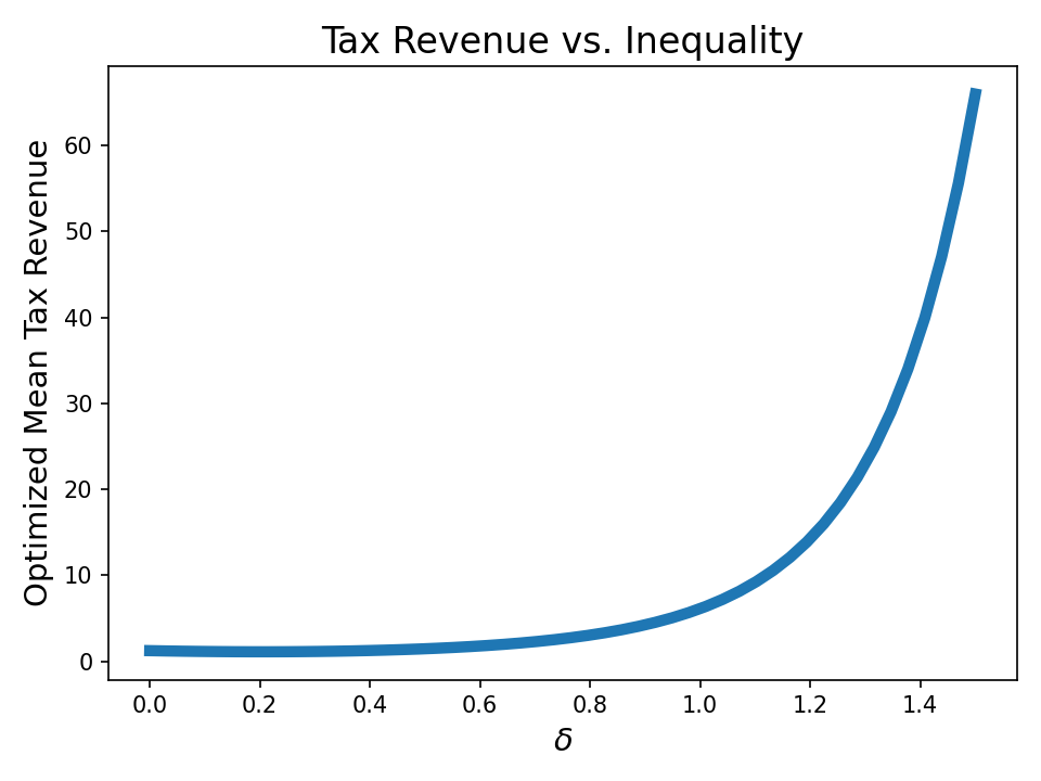
Interestingly, the greater the skill inequality, the more the poorest people get – even when fixing the average amount of skill. You might be thinking “Well I don’t like this – somehow those fancy high-skill workers are somehow still getting all the money!”
But if you look at what’s actually happening, we basically have a bunch of high-skill adderalled techbro slaves pulling 23 hour days. These guys make insane salaries, but only keep a small fraction of what they earn. All the rest gets given to non-workers, who chill on the beach all day drinking margaritas.
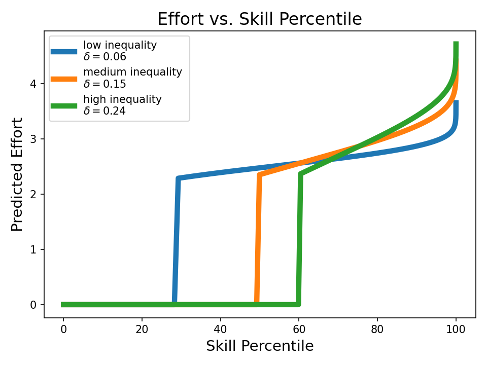
As we increase the inequality, a higher fraction of people no longer work. Meanwhile, those at the highest skill levels work even harder.
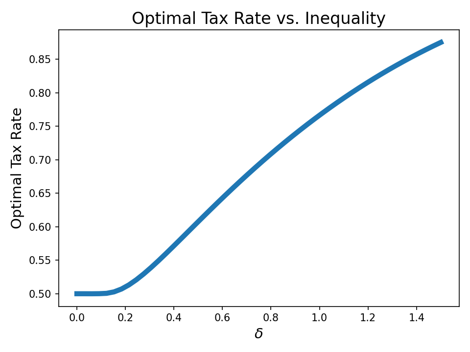
Where is all that income going?
Well if we look at the tax rate, it’s being taken by the government – and given to everyone.
In conclusion, I have no idea at all what any of all this actually means. I don’t even know whether I’m describing a utopia or a dystopia.
But it’s at least satisfying to be able to produce a Laffer curve using something other than a napkin and common sense.