
A while ago my friend Chad suggested that we make algorithms to play battleship on sets of random boards and see whose was better. This was all inspired by a blogpost Chad had read from datagenetics, where Nick Berry applied battleship algorithms to random boards and saw which ones worked better than others.
I only had a few free hours, so I decided that I wanted to make an algorithm that was as good as possible, under the strict constraint that it was also as dumb as possible. I wanted to avoid complicated math, difficult combinatorics, and any algorithm that would require walking down some huge decision tree I would have to manually populate.
As basic as the underlying idea was, the project raised a number of interesting ideas, and put the pros and cons of neural networks (NNs) in sharp relief.
As the datagenetics blogpost concludes, a really good battleship algorithm would be one which takes in the current state of the board – the squares where it sees a ship, the squares where it sees ocean, and the squares it has not attacked yet – and uses it to determine the probability that each unattacked square has a ship on it. It then goes through those unattacked squares, and chooses the most probable one to be its next target.
This is a pretty dumb greedy algorithm, so I’m not totally sure its optimal – it’s conceivable that the optimal algorithm might also target squares based on which one maximally informs it about the positions of ships (some kind of explore vs exploit issue). But this is precisely the kind of question I don’t want to think about here.
The hard part is generating a function from board state to probabilities. The first ‘dumb’ answer that comes to mind to solve this would be to just use Monte Carlo.
Under a Monte Carlo algorithm, I start with my partially explored board, where every unexplored square has a value of zero. I then place the ships that remain undiscovered in some random configuration such that they fit. I record where the ships were, adding 1/N to the value of each square they occupy, and remove the ships. If I do this whole process N»1 times, I should get a pretty good probability function telling me how likely each square is to have a ship on it.
Immediately this is too complicated for me.
I would have to take a given board state (for example, the board below), and generate thousands of boards which matched my current knowledge. For me, that’s too much.
Ideally, I would just have a function that takes in knowledge about a board and outputs a probability distribution. Why don’t we use a neural network to try to get something close to this.
Here is the idea: Train a neural network on partially explored battleship boards with the goal of having it output a probability density function for the output board.
The Neural Network (NN)
Here the data comes in the form of images of the board’s state, with each ‘pixel’ being either hit, miss, or unknown. These images contain features that are to a degree translationally invariant – the same arrangement of ships can be shifted around the board. There are also certain small-scale features of the images that can tell us about the underlying arrangement of ships. The feature of a ‘hit’ with unexplored squares all around tells us that a ship is either to left of it, right of it, above it, or below it.
This type of input data is perfect for particular type of NN known as convolutional. These NNs apply convolutions to an image using many different kernels. The kernels evolve during training and, once optimized, tend to pick out important features of the input image.
To keep things simple, I used the neural network architecture shown below (right now I’m taking outputs to be logits):
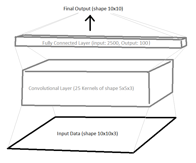
We have one convolutional layer (no max pooling or anything – I want this as simple as possible) and one fully connected layer (both with Relu activation). We get our probability distribution output by reshaping from a length 100 list to a 10x10 array.
There’s also some obvious symmetry available to us here. Obviously if I flip any board, my predictions should be the same (but flipped). The same applies to rotations of the board. Collectively these make up the dihedral group, $D_4$, which has 8 elements: 4 rotations by $\pi/2$, and 4 rotations with a flip included. We therefore want our probabilities to be invariant under $D_4$:
\[p(\hat{O} board) = p(board) \forall \hat{O} \in D_4\]To ensure this, I’ll define the total output of the model to be
\[NN(board) = \frac{1}{8} \sum_{\hat{O} \in D_4} \tilde{NN}(\hat{O} board)\]Where I’ve used $\tilde{NN}$ to refer to a single unsymmetrized evaluation of the network. Above, I’m averaging logits – to get a probability apply a sigmoid to the averaged logits. Intuitively, applying a sigmoid after averaging should allow the symmetries to improve learning.
Next we need to train the NN. We want the input data to be the types of board states the NN will likely see during gameplay – partially revealed boards with hits and misses according to the history of the game. The labels for this data would then be the true states of the boards. During training, we teach the NN to use the board states with the correct underlying board.
Then as the NN plays battleship, it will see the types of boards it was trained on and will be able to use these to predict where the ships are and are not.
There is a slight problem here: the boards the NN will see during gameplay are precisely the boards an optimized NN algorithm will naturally lead itself to. How can we pick the right board states to train the NN, if the boards we want are precisely those that we need a trained NN to obtain? (what a confusing sentence)
The First Born Approximation
This same type of issue comes up in physics often. In particular, we see this in the problem of a plane wave hitting a potential and scattering off. If we go through the math of this problem we end up with the following formula:
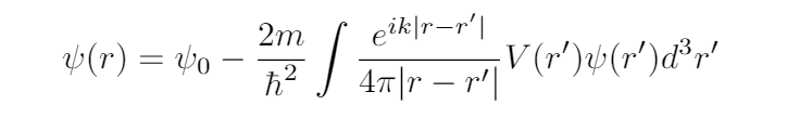
Our goal is to solve for $\psi(r)$, the scattered wave.
To find $\psi(r)$, we must evaluate the right hand side. But to evaluate the right hand side, we already need to know $\psi(r)$. The way physicists get around this is to assume that $\psi(r)$ will be something like the plane wave, $\psi_{0}(r)$. So we replace $\psi(r’)$ on the right hand side with $\psi_{0}(r’)$. We can then evaluate this and obtain what is known as the First Born Approximation, written $\psi_{1}(r)$.
We say ‘First’ because in principle I can do this as many times as I want. Replacing $\psi$ in the right hand side of our equation with $\psi_{1}$ and evaluating gives us the second Born approximation, $\psi_{2}$, and so on.
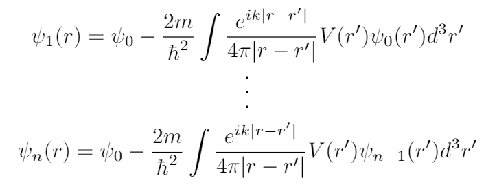
The idea is that if our initial guess of a plane wave is sufficiently close to the right answer, repeated application of this algorithm will make $\psi_{n}$ converge correctly to $\psi$.
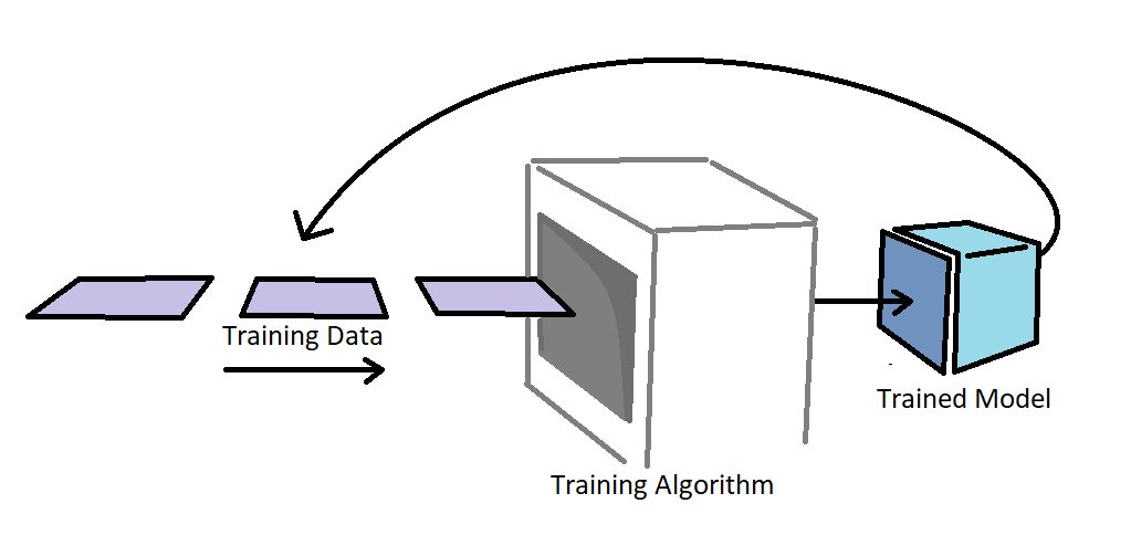
Let’s get back to the problem of getting data to train the NN model. If we wrote it in the form of an equation, we would have something like:

That is, the trained model comes from taking an untrained model, and applying the training algorithm (which itself requires the trained model to generate training data).
We can approach this from exactly the same Born mentality as before: assume that the strategy of the trained model will be in some way a variation of the strategy of the untrained model (random guessing). We can then write what I will call the First Born Approximation of the NN model.

Now, again, if I really wanted to I could keep going and instead get the second, third, or fourth Born Approximations of the NN. The reasons not to do this are, however, extremely compelling:
- I don’t care nearly enough to do it.
- The whole point of this was to make it simple.
- I reeeeaaally don’t want to do it.
Great! Now I have a neural network that has been trained to take as an input some partially explored board, and give as an output an entire board with each square getting a number between 0 and 1. The greater the number, the more likely the square is to be occupied.
Are Outputs Probabilities?
This brings up a subtle question. How do I know I can interpret these numbers as probabilities? At this point all I know is that if my neural network is perfect, then the more likely a square is to be occupied, the closer the NNs output for that square is to 1. But does this mean the outputs are necessarily probabilities? Not at all.
Really, all I can know is that my NN produces some monotonically increasing function of the probability.
There are two responses to this concern:
1.
I don’t care. All I care about is choosing the most probable unexplored square. So as long as the output of the neural network is a strictly increasing function $f$ of the actual probability, our choice of most probable next square is unchanged and our algorithm stays the same.
\[max(\{ p(x_{i, j}) | x_{i, j} \in unexplored \}) = max(\{ f(p(x_{i, j})) | x_{i, j} \in unexplored \})\]2.
If you’re really invested in this question, there is a way to make sure that the neural network’s output corresponds to its internal probabilities and not just some monotonic function of them.
The output of a neural network depends on the loss function that it is trained with. Essentially, this is the function used to determine the difference between the correct probability distribution and the one the NN produced. It tells the algorithm how ‘incorrect’ the NN is, and the algorithm tries to minimize it.
So which loss function forces the NN to tell us the probabilities themselves? [The derivation I give is mostly lifted from a Terry Tao blogpost about a related topic].
Let $p(x_{i, j})$ be the probability that the square at (i, j) is occupied, and let $q(x_{i, j})$ be the output that the NN actually gives for that square.
Then the loss function we want would be the function, $L$, such that the expected loss
\[p(x_{i, j}) L(1, q(x_{i, j}))+(1-p(x_{i, j})) L(0, q(x_{i, j}))\]is minimized when $q(x_{i, j})=p(x_{i, j})$.
This can be read as “(the probability of being correct) times (the loss if correct) plus (the probability of being incorrect) times (the loss if incorrect)”
To simplify things, we can see that $L(0, q(x_{i, j})) = L(1, 1-q(x_{i, j}))$. In words: the punishment for having the output be 0, when you predicted it would be 1 with probability $q(x_{i, j})$ should be the same as the punishment for having the output be 1 when you said it would be zero with probability $1 - q(x_{i, j})$.
Using this, we can make things more concise and say that $L$ must minimize
\[p(x_{i, j}) L(q(x_{i, j}))+(1-p(x_{i, j})) L(1 - q(x_{i, j}))\]When $q(x_{i, j})=p(x_{i, j})$.
We ensure this by setting the derivative with respect to $p(x_{i, j})$ to zero at $q(x_{i, j})=p(x_{i, j})$. That is:
\[0 = p(x_{i, j}) L'(p(x_{i, j})) - (1-p(x_{i, j})) L'(1 - p(x_{i, j}))\]This is solved by $L( p ) = - Log( p )$, which is equal to a loss function known as cross entropy. Cross entropy, it so happens, is exactly the function my training algorithm uses to compare the NN output to the actual board.
If we let ocean squares = 0, and squares with ships = 1, then the full boards we train our NN on are already probability distributions, $p(x_{i, j})$. Using the cross entropy loss function during this training will then force our outputs to be probabilities! (again, not that we care)
Once training is done, we have our algorithm!
Now we just have to do some analysis to see how good (or shitty) it is.
Watching the Game
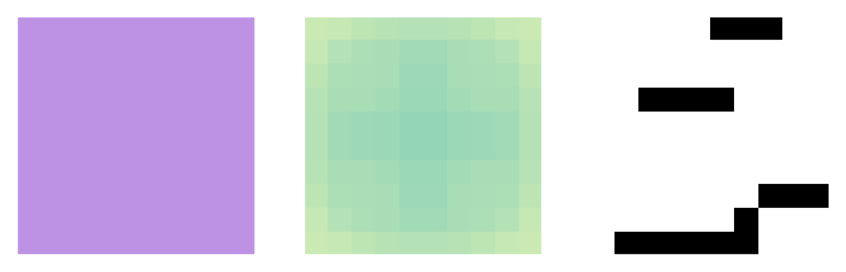
First, just for fun, lets see how a typical board is played.
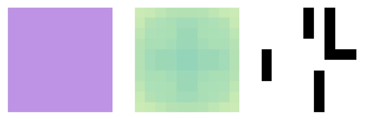
To the left we have the actual gameplay, with purple representing an unknown square, white a miss, and black a hit. To the upper right, we have the NNs internal probability distribution (darker = more likely to be a ship), and to the lower right we have the actual board.
There’s a lot of remarkable stuff going on in this game, and much of it is surprisingly intuitive. When we watch the algorithm play, it seems almost human in how it appears to be gaining an internal understanding of the board.
We see that when the NN gets a hit or a miss, the probability distribution suddenly gets a vertical and horizontal streak centered at that point.
If it’s a hit, then the NN tends to follow these dark probability streaks until it understands that either it’s searching in the wrong direction, or its found all of the ship.
The NN also understands the directionality of the ships it sees. It always seems to make sure that both ends of a line of hits are unoccupied before moving on, but it doesn’t really care about the immediate ‘left’ and ‘right’ of these hits, as we see when the NN attacks the vertical ship in the above game. Clearly it understands the general shapes of the ships on the board.
Data Analysis
Let’s move on to an analysis that’s more quantitative: the distribution of the lengths of a different games. I let my algorithm run for a while, and after around 2500 games I checked the distribution of how long they tended to take.
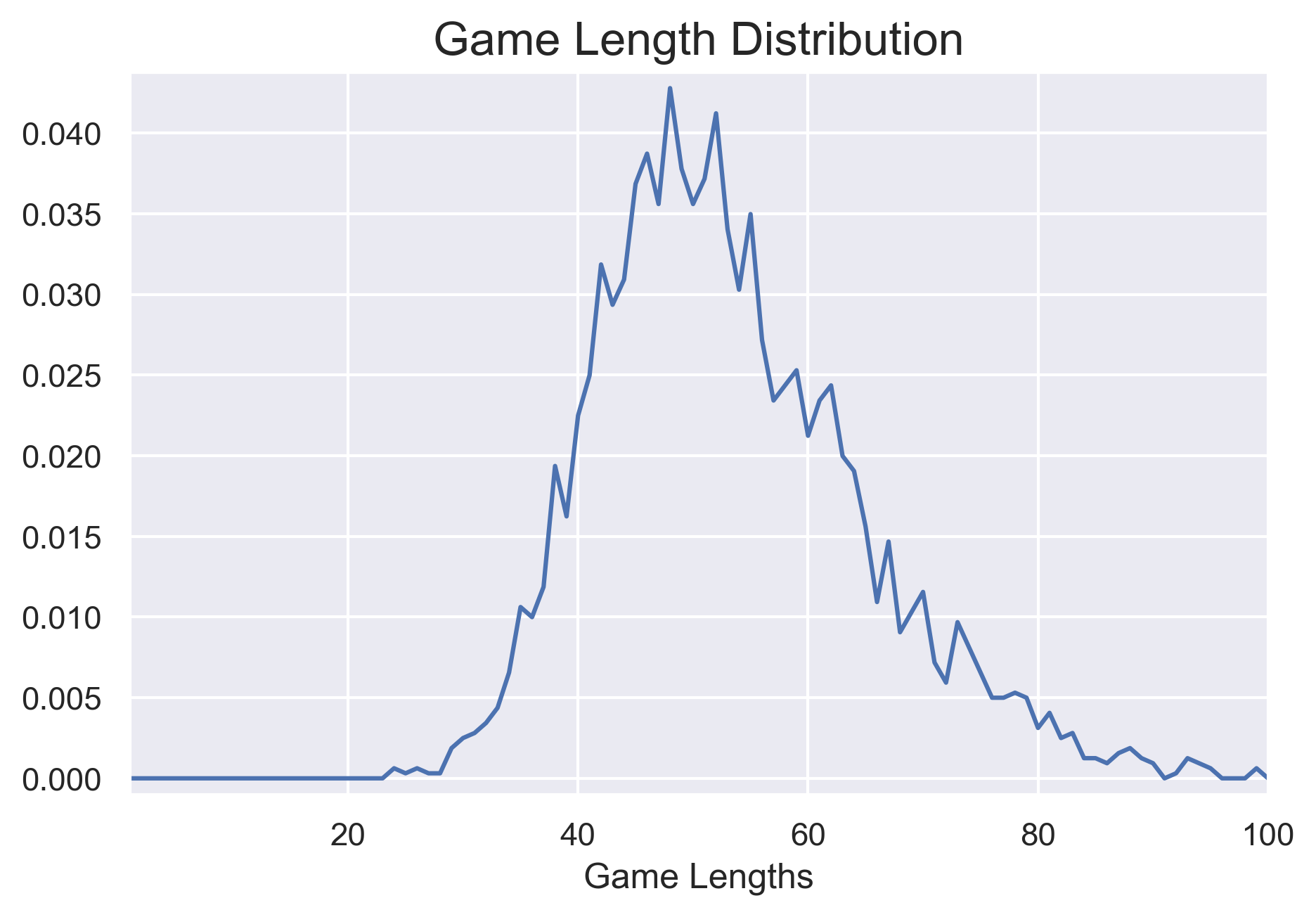
The median here (i.e. the number of moves needed to win at least half the games) was 52. But how does this compare?
This quantity is something that Nick Berry analyzed in his blog for four different algorithms: one that uses the exact probability, two custom algorithms of his own design, and one that chooses random squares until it wins.
Below we show the fraction of games won as a function of the number of moves made. The dotted red line is my algorithm’s median, and the other vertical lines are the medians of Nick Berry’s algorithms.

My algorithm was vastly better than random and also beat out both of his custom algorithms. Unfortunately, it was about 10 moves behind his probabilistic algorithm, but for not really trying too hard on perfecting this, I don’t feel too bad about that.
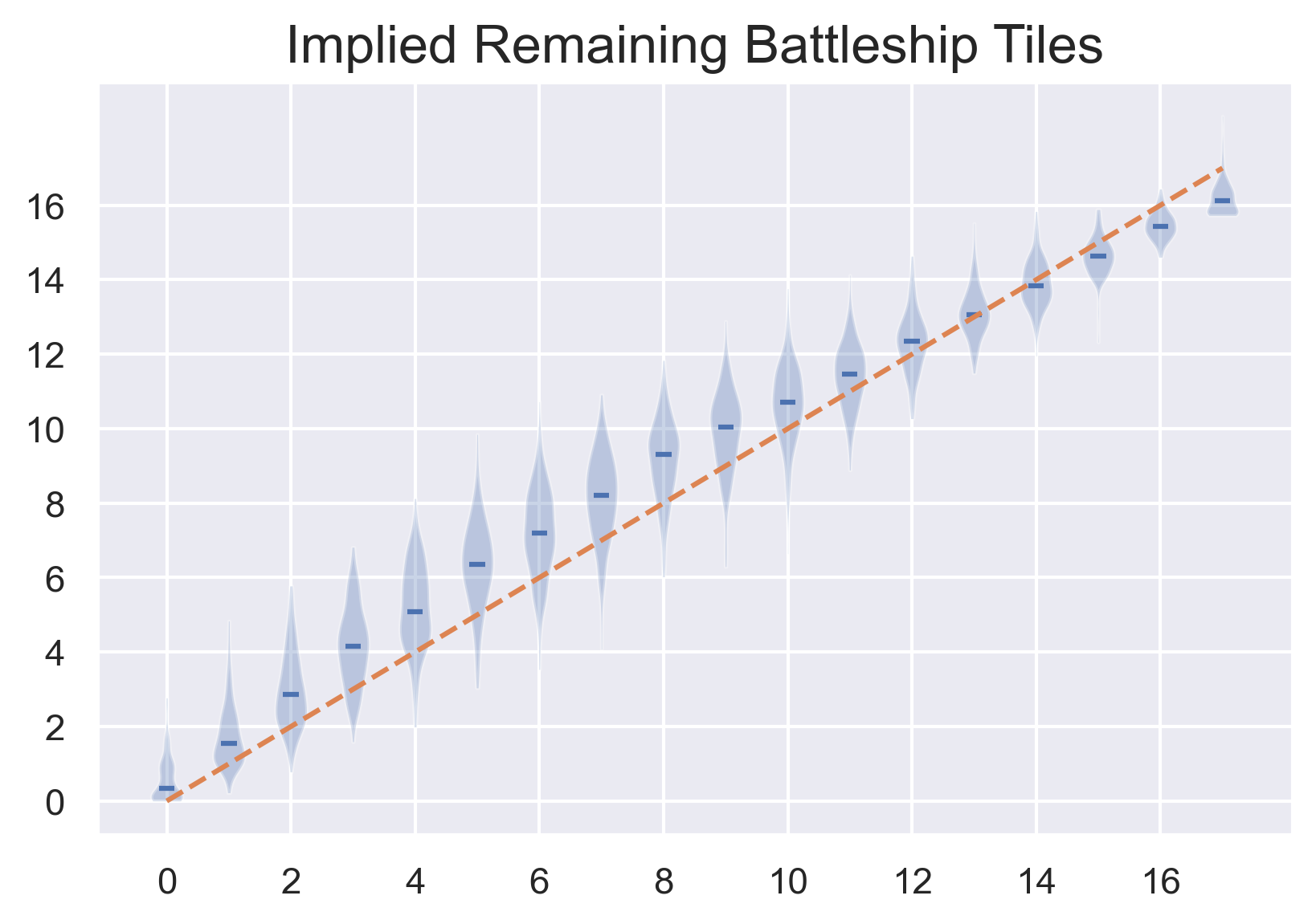
Another interesting analysis shows that my algorithm even ‘knows’ how many ships it has left to find. I applied my algorithm to some partially revealed random boards (the same type used as training data). Then I summed up the probability that the algorithm gave for each unexplored square to have a ship on it, and compared this number with the actual number of squares with ships left to be found. The two sets of numbers line up almost exactly.
We can also easily see that there are some serious problems with this algorithm. For instance, if we look at the game length distribution, we see that there was at least one game which took around 98 moves.
This really makes no sense, since in theory one could simply attack squares in a checkerboard pattern and then fill squares in to finish off the ships. Even this very inefficient algorithm would complete a game in much less than 98 moves.
To find out what’s going on here, we can look at an especially long game and see what mistakes it makes.
This game took literally 100 moves – way longer than any human would ever take, and longer than random guessing (on average). The cause of this failure is the long piece placed horizontally at the bottom of the board, which has a little 2-square boat rotated vertically at its right end. This utterly baffles the neural network, and it ends up predicting that it’s more likely that a ship is on a single isolated square (which is impossible) than it is for a tile to be occupied above the long stretch of hits. Obviously the single set of convolutional filters alone aren’t a replacement for reasoning.
Let’s see how the algorithm plays during one of its faster games, this one taking just 19 moves.

Clearly things are easier in a game of battleship when ships are touching each other and in the center of the board.
Finally, heres a ‘median game’ taking around 52 moves
Potential Improvements
(skip if you don’t care)
I can immediately see two ways that it would be possible to improve this algorithm.
-
Include some hard logic. After telling my friend Chad about the algorithm, he reminded me that in the actual game you get told when you sink a ship. Clearly this information should inform the model of the board, and currently it doesn’t.
-
I could go to a higher ‘Born approximation’ of the NN. This would probably improve performance, but it wouldn’t be very fun to do.
Final Thoughts
The weaknesses of this algorithm stem from the same quality that provides so much strength – its use of fast heuristics over some protracted application of logic.
Humans aren’t natural logicians. Instead, we use sets of heuristics to analyze the different patterns we come across. This is exactly what neural networks do as well (remember, our brains are (spiking) neural networks). Neural networks are effective because they’re able to find good internal representations of the various patterns observed in the data, and (in supervised learning) learn to correlate these with the training labels.
My NN could have learned to give zero probability to the unexplored squares surrounded by misses. The fact that it doesn’t do this is likely a result of the Born approximation we applied, resulting in a lack of this pattern in the training data.
But that the NN was so smart in some ways, but so dumb in this way, really exemplifies the fact that it is not using reason, and it is not able to extrapolate using logic. Humans need intense training to be able to algorithmically apply logic using our heuristic brains, and neural networks are largely the same.
This neural network is simply pattern matching over the landscape of data it has been trained on, and it is unable to stretch its ‘understanding’ beyond that. [Insert allusion to the human experience here]
A note: I originally wrote this back in 2018. Back then I was using tensorflow (1) – with sessions and all that. I rewrote it though when I went through this post, and to preserve historicity, I used tensorflow 2.